RSSA file

The complete API can be found at f4enix.output.rssa.RSSA

MCNP allows to record particles crossing a surface during a Monte Carlo simulation in order to use them as a source in a subsequent analyses. These particle tracks are stored in a file called RSSA.

Loading and analyzing a RSSA file

The binary reader of this tool is very fast as it has been vectorized via Numpy. Reading a RSSA file of 6 Gb with the PyNE reader takes around 15 minutes while this reader does the same in 10 seconds. Lets start by loading a new RSSA file.

from matplotlib import pyplot as plt

from f4enix.core.egroups import GROUP_STRUCTURES
from f4enix.output.rssa import RSSA, PlotParameters, SpectraPlotParameters

# The class is initialized by providing the path to the file
my_rssa = RSSA.read_from_file("small_cyl.w")
my_rssa  # printing shows relevant information

/home/docs/checkouts/readthedocs.org/user_builds/f4enix/envs/developing/lib/python3.10/site-packages/tqdm/auto.py:21: TqdmWarning: IProgress not found. Please update jupyter and ipywidgets. See https://ipywidgets.readthedocs.io/en/stable/user_install.html
  from .autonotebook import tqdm as notebook_tqdm

RSSA file was recorded using the following surfaces:
  Surface ID: 1, type: 1
The total number of tracks recorded is 72083.
Neutrons: 72083 photons: 0, The simulation that produced this RSSA run 100000 histories.
The amount of independent histories that reached the RSSA surfaces was 70797.

my_rssa.tracks  # This is an array containing all the infomation of all the tracks
my_rssa.x  # With this command we acces a vector holding the X position of every track
my_rssa.y  
my_rssa.z  # Same for Y and Z coordinates and the Weight values of the tracks
my_rssa.wgt
my_rssa.energies
my_rssa.histories  # History number of the tracks

# Lets print some information of the 1234 track recorded in the RSSA file
index = 1234
position = (my_rssa.x[index], my_rssa.y[index], my_rssa.z[index])
print(f'The track with index {index} was recorded at position:\n{position}')
print(f'The track had an energy of {my_rssa.energies[index]} MeV and weight of {my_rssa.wgt[index]}')
print(f'The track was originated at the history number {my_rssa.histories[index]}')

The track with index 1234 was recorded at position:
(-0.13126632308094988, 29.99971281783252, 12.254586722666627)
The track had an energy of 14.0 MeV and weight of 1.0
The track was originated at the history number -1739

The RSSA file may contain both neutrons and photons. The tool has a way to easily dicriminate between particle types with the use of filters, also called masks.

Plot cylindrical surfaces

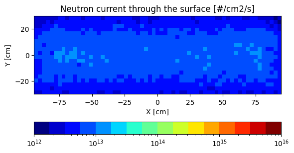
The level of customization possible with these type of plots is quite high.

# Plot the neutron current
(
    my_rssa.plot_cyl()
    .set_particle("n")  # Only neutrons will be plotted
    # .set_surface_ids([1])  # We can use many functions to customize the plot
    .set_z_limits(-600, 800)
    .set_perimeter_limits(-500, 1000)
    .calculate_bins(bin_width=3)  # Set the width of the bins to 3 cm
    .get_particle_current(1e17)  # Make the plot for current with 1e17 n/s
    .set_plot_parameters(
        PlotParameters(
            vmin=1e12,
            vmax=1e16,
            number_of_colors=16,
            legend_orientation="horizontal",
            title="Neutron current through the surface [#/cm2/s]",
        )
    )
    # .save_figure("bioshield_current_be_1e14.png")  # Save the figure to a file
    .show()  # Simply show the figure to a window instead of saving it
)

<f4enix.output.rssa.rssa_plotting.RSSAPlot at 0x7aaef899a650>

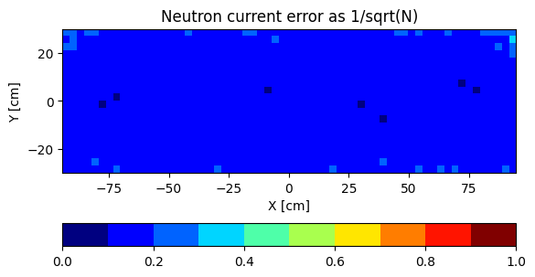
# Plot the neutron current statistical errors
(
    my_rssa.plot_cyl()
    .set_particle("n")  # Only neutrons will be plotted
    # .set_surface_ids([1])  # We can use many functions to customize the plot
    .set_z_limits(-600, 800)
    .set_perimeter_limits(-500, 1000)
    .calculate_bins(bin_width=3)  # Set the width of the bins to 3 cm
    .get_particle_current_errors()
    .set_plot_parameters(
        PlotParameters(
            vmin=0,
            vmax=1,
            number_of_colors=10,
            norm="linear",
            legend_orientation="horizontal",
            title="Neutron current error as 1/sqrt(N)",
        )
    )
    # .save_figure("bioshield_current_be_1e14.png")  # Save the figure to a file
    .show()  # Simply show the figure to a window instead of saving it
)

<f4enix.output.rssa.rssa_plotting.RSSAPlot at 0x7aaef14b5a20>

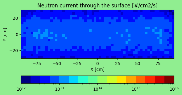
But if it was not sufficient it is possible to act on the matplotlib figures directly:

fig, ax = (
    my_rssa.plot_cyl()
    .set_particle("n")  # Only neutrons will be plotted
    # .set_surface_ids([1])  # We can use many functions to customize the plot
    .set_z_limits(-600, 800)
    .set_perimeter_limits(-500, 1000)
    .calculate_bins(bin_width=3)  # Set the width of the bins to 3 cm
    .get_particle_current(1e17)  # Make the plot for current with 1e17 n/s
    .set_plot_parameters(
        PlotParameters(
            vmin=1e12,
            vmax=1e16,
            number_of_colors=16,
            legend_orientation="horizontal",
            title="Neutron current through the surface [#/cm2/s]",
        )
    )
    # .save_figure("bioshield_current_be_1e14.png")  # Save the figure to a file
    .get_plot()
)
fig.patch.set_facecolor("lightgreen")  # Set the figure background color
plt.show()

Plot RSSA spectra

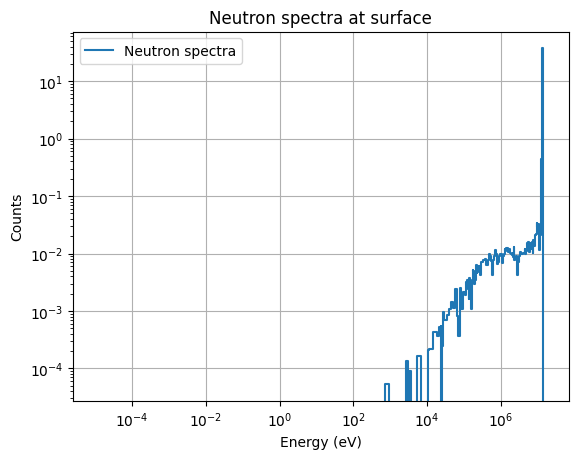
The plotting of RSSA spectra is also possible with a high level of customization.

Please consider that:

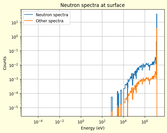
• The spectra is calculated by grouping by energy bins the particles, the statistical weight of each particle is summed in each bin.

• The Y-Axis is counts per unit of lethargy.

• The counts are normalized to 1 (unit area below the curve).

• The spectra is presented in a loglog scale.

• By default the energy bins employ the VITAMIN-J structure. Can be changed via the set_energy_bins method.

(
    my_rssa.plot_spectra()
    .set_particle("n")
    .set_z_limits(-600, 800)
    .set_energy_bins(GROUP_STRUCTURES["VITAMIN-J-175"])
    .set_plot_parameters(
        SpectraPlotParameters(
            title="Neutron spectra at surface",
            xlabel="Energy (eV)",
            ylabel="Counts",
            label="Neutron spectra",
        )
    )
    # .save_figure(tmp_path / "test_plot_spectra.png")  # Save the figure to a file
    .show()  # Simply show the figure to a window instead of saving it
)

<f4enix.output.rssa.rssa_plotting.RSSASpectraPlot at 0x7aaef03c5de0>

It is possible to combine multiple RSSA spectra files in the same plot or show the result of different filtering strategy.

other_spectra = (
    my_rssa.plot_spectra()
    .set_particle("n")
    .set_z_limits(-600, 800)
    .set_energy_bins(GROUP_STRUCTURES["VITAMIN-J-175"])
    .set_plot_parameters(
        SpectraPlotParameters(
            label="Other spectra",
        )
    )
    .get_spectra_info()
)
other_spectra.normalized_counts *= 0.1  # Just to differentiate the plots
fig, _ax = (
    my_rssa.plot_spectra()
    .set_particle("n")
    .set_z_limits(-600, 800)
    .set_energy_bins(GROUP_STRUCTURES["VITAMIN-J-175"])
    .set_plot_parameters(
        SpectraPlotParameters(
            title="Neutron spectra at surface",
            xlabel="Energy (eV)",
            ylabel="Counts",
            label="Neutron spectra",
        )
    )
    .get_combined_plot_with_other_spectras(other_spectra)
)
fig.patch.set_facecolor("lightyellow")  # Set the figure background color
plt.show()

Managing very large files

RSSA files can become very large (100+ Gb). These files may not fit in the memory of the computer. For that reason, the scan_tracks methods has been developed. It returns a LazyFrame instead of a DataFrame. This allows the reading of the file in batches but also the use of polars expressions to filter the data before loading it in memory. This way we can load only the data we are interested in and not the whole file.

import polars as pl

from f4enix.output.rssa.rssa_reader import parse_header, scan_tracks

file_parameters = parse_header("small_cyl.w")
# Modify the default batch size in this function depending on your memory capabilities
lazy_tracks = scan_tracks("small_cyl.w", default_batch_size=10_000_000)

# We can read only the first N tracks of the file immediately before deciding on more
# advanced filters
first_5_tracks = lazy_tracks.head(5).collect()
print(first_5_tracks)

shape: (5, 11)
┌─────┬─────┬──────────┬───────────┬───┬────────────┬───────────┬───────────┬─────┐
│ a   ┆ b   ┆ wgt      ┆ erg       ┆ … ┆ z          ┆ u         ┆ v         ┆ c   │
│ --- ┆ --- ┆ ---      ┆ ---       ┆   ┆ ---        ┆ ---       ┆ ---       ┆ --- │
│ i64 ┆ i64 ┆ f64      ┆ f64       ┆   ┆ f64        ┆ f64       ┆ f64       ┆ i64 │
╞═════╪═════╪══════════╪═══════════╪═══╪════════════╪═══════════╪═══════════╪═════╡
│ 2   ┆ 8   ┆ 0.979868 ┆ 13.550991 ┆ … ┆ 5.162862   ┆ 0.573595  ┆ -0.782844 ┆ 0   │
│ -3  ┆ 8   ┆ 1.0      ┆ 14.0      ┆ … ┆ 25.294793  ┆ -0.618427 ┆ -0.449477 ┆ 0   │
│ 4   ┆ 8   ┆ 0.979868 ┆ 13.596932 ┆ … ┆ -19.163922 ┆ 0.727551  ┆ -0.092989 ┆ 0   │
│ -9  ┆ 8   ┆ 1.0      ┆ 14.0      ┆ … ┆ -9.707136  ┆ -0.236817 ┆ 0.921489  ┆ 0   │
│ -11 ┆ 8   ┆ 1.0      ┆ 14.0      ┆ … ┆ -5.822491  ┆ -0.66983  ┆ -0.717654 ┆ 0   │
└─────┴─────┴──────────┴───────────┴───┴────────────┴───────────┴───────────┴─────┘

# We can build an RSSA object taking all the tracks that fulfill a filtering expression
filtered_tracks = (
    lazy_tracks.drop(["u", "v", "a", "tme"])
    .filter(pl.col("wgt") < 1.0)
    .filter(pl.col("x") > 0)
).collect()

custom_rssa = RSSA(file_parameters, filtered_tracks)
# custom_rssa.save_to_files("path_to_folder")
# loaded_rssa = RSSA.load_from_saved_files("path_to_folder")

print(custom_rssa.tracks)

shape: (4_490, 7)
┌─────┬──────────┬───────────┬───────────┬────────────┬────────────┬─────┐
│ b   ┆ wgt      ┆ erg       ┆ x         ┆ y          ┆ z          ┆ c   │
│ --- ┆ ---      ┆ ---       ┆ ---       ┆ ---        ┆ ---        ┆ --- │
│ i64 ┆ f64      ┆ f64       ┆ f64       ┆ f64        ┆ f64        ┆ i64 │
╞═════╪══════════╪═══════════╪═══════════╪════════════╪════════════╪═════╡
│ 8   ┆ 0.979868 ┆ 13.550991 ┆ 20.858324 ┆ -21.562243 ┆ 5.162862   ┆ 0   │
│ 8   ┆ 0.979868 ┆ 13.596932 ┆ 29.855251 ┆ -2.943469  ┆ -19.163922 ┆ 0   │
│ 8   ┆ 0.914503 ┆ 4.688492  ┆ 22.458954 ┆ -19.88958  ┆ 3.333919   ┆ 0   │
│ 8   ┆ 0.966763 ┆ 0.570175  ┆ 22.557919 ┆ -19.777267 ┆ -2.555544  ┆ 0   │
│ 8   ┆ 0.960412 ┆ 7.01652   ┆ 29.460265 ┆ 5.665051   ┆ -3.958737  ┆ 0   │
│ …   ┆ …        ┆ …         ┆ …         ┆ …          ┆ …          ┆ …   │
│ 8   ┆ 0.979868 ┆ 13.949697 ┆ 29.728642 ┆ 4.025897   ┆ -4.338646  ┆ 0   │
│ 8   ┆ 0.979868 ┆ 13.58059  ┆ 27.518898 ┆ -11.94614  ┆ -6.107839  ┆ 0   │
│ 8   ┆ 0.979868 ┆ 1.675429  ┆ 24.225364 ┆ -17.695528 ┆ -15.579247 ┆ 0   │
│ 8   ┆ 0.979868 ┆ 11.392901 ┆ 28.96016  ┆ -7.830015  ┆ -7.329891  ┆ 0   │
│ 8   ┆ 0.941852 ┆ 13.263379 ┆ 24.570253 ┆ 17.213444  ┆ 18.129407  ┆ 0   │
└─────┴──────────┴───────────┴───────────┴────────────┴────────────┴─────┘