
MESHTAL file#
The complete API can be found at f4enix.output.meshtal.Meshtal
It is possible to parse and MCNP meshtal file and obtain a pyvista object for each of the fmeshes.
# import the related module and parse a meshtal file
from f4enix.output.meshtal import Meshtal

# file = 'mode0_plasma_prod.msht'
file = 'meshtal'
meshtal = Meshtal(file)

# By default all meshes are parsed, but if speed up is needed, only a subset
# of them can be selected
meshtal.readMesh()
meshtal
/home/docs/checkouts/readthedocs.org/user_builds/f4enix/envs/developing/lib/python3.10/site-packages/tqdm/auto.py:21: TqdmWarning: IProgress not found. Please update jupyter and ipywidgets. See https://ipywidgets.readthedocs.io/en/stable/user_install.html
  from .autonotebook import tqdm as notebook_tqdm
<f4enix.output.meshtal.meshtal.Meshtal at 0x778e79e09210>
import tempfile  # To have a scratch directory for the example
outpath = tempfile.gettempdir()

# fmeshes can be dumped all together
meshtal.write_all(outpath, out_format='vtk')

# Or specifically with higher control
meshtal.mesh[1004].write(outpath, list_array_names=['Value - Total'],
                         out_format='ip_fluent', outfile='custom name')
Writing x: 0%| | 0/1000 [00:00<?, ? x points/s]
Writing x: 100%|██████████| 1000/1000 [00:00<00:00, 100868.26 x points/s]
Writing y: 0%| | 0/1000 [00:00<?, ? y points/s]
Writing y: 100%|██████████| 1000/1000 [00:00<00:00, 94440.78 y points/s]
Writing z: 0%| | 0/1000 [00:00<?, ? z points/s]
Writing z: 100%|██████████| 1000/1000 [00:00<00:00, 103414.96 z points/s]
Writing values: 0%| | 0/1000 [00:00<?, ? values/s]
Writing values: 100%|██████████| 1000/1000 [00:00<00:00, 1027260.35 values/s]
instead of writing them all separate it could be useful to collapse all fmeshes into a single pyvista grid. This is possible only if the fmeshes have the same geometry and have no binning.
# this dictionary provides the names for the value and error in each fmesh
dict_names = {1004: ['neutron flux', 'neutron flux err'],
              1024: ['photon flux', 'photon flux err']}
collapsed_grid = meshtal.collapse_grids(dict_names)
collapsed_grid
RectilinearGrid (0x778e3c32bca0)
  N Cells:      1000
  N Points:     1331
  X Bounds:     -1.300e+03, 1.300e+03
  Y Bounds:     -1.300e+03, 1.300e+03
  Z Bounds:     -9.000e+02, 9.000e+02
  Dimensions:   11, 11, 11
  N Arrays:     4
# select a specific fmesh.
n_flux_fmesh = meshtal.mesh[1004]

# Access the related pyvista object and all its powerful methods
# The units from MCNP apply if no modification is made by the user
n_flux = n_flux_fmesh.grid
n_flux
RectilinearGrid (0x778e3c32ba00)
  N Cells:      1000
  N Points:     1331
  X Bounds:     -1.300e+03, 1.300e+03
  Y Bounds:     -1.300e+03, 1.300e+03
  Z Bounds:     -9.000e+02, 9.000e+02
  Dimensions:   11, 11, 11
  N Arrays:     2
import pyvista as pv

try:
    pv.start_xvfb()
except (OSError, AttributeError):
    # this is needed only on Linux headless servers
    pass
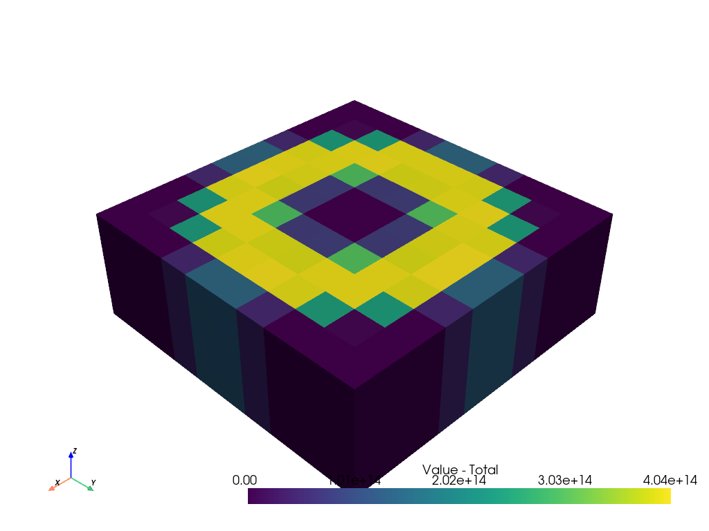
# quick plot to check that the meshes are not empty
clip = n_flux.clip(normal='z')  # native pyvista clip
clip.plot(scalars='Value - Total', jupyter_backend='static')
2026-05-19 11:11:27.336 ( 0.944s) [ 778E8E0BFB80]vtkXOpenGLRenderWindow.:1460 WARN| bad X server connection. DISPLAY=
import pyvista as pv

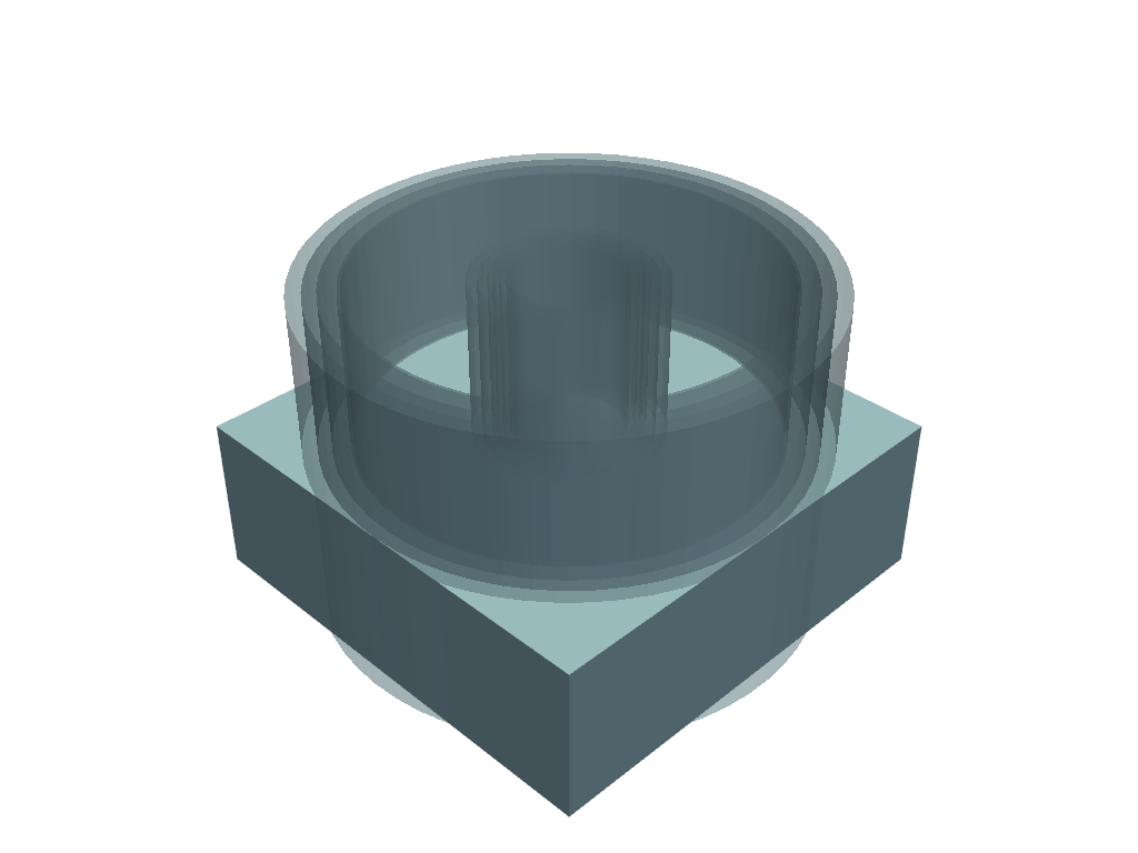
# Load an .stl file to be used for plots and plot them with the fmesh to check
# that the units match. stl units will depend by export settings of the user
stl = pv.read('iter1D.stl').scale(10)  # scale the stl to have same units

# Set up and show a pyvista plotter
plotter = pv.Plotter()
plotter.add_mesh(clip)
plotter.add_mesh(stl, opacity=0.4)
plotter.show(jupyter_backend='static')
# Load additional modules related to Atlas production
from f4enix.output.plotter import MeshPlotter, Atlas
from copy import deepcopy

# Get a basic PyVista mesh where to store all other data
global_mesh = deepcopy(meshtal.mesh[1004].grid)

# On the same grid, load all the different fmeshes results. In this case there
# are only two
for tally_num, fmesh in meshtal.mesh.items():
    # get the FC card comment for the fmesh to be used as name of the scalar
    name = fmesh.comments.strip()
    # get the scalar values
    data = fmesh.grid['Value - Total']
    # Adding the array to the global mesh
    global_mesh[name] = data

# Clean the original results from the template mesh
global_mesh.cell_data.remove('Value - Total')
global_mesh.cell_data.remove('Error - Total')

global_mesh
RectilinearGrid (0x778e36797880)
  N Cells:      1000
  N Points:     1331
  X Bounds:     -1.300e+03, 1.300e+03
  Y Bounds:     -1.300e+03, 1.300e+03
  Z Bounds:     -9.000e+02, 9.000e+02
  Dimensions:   11, 11, 11
  N Arrays:     2
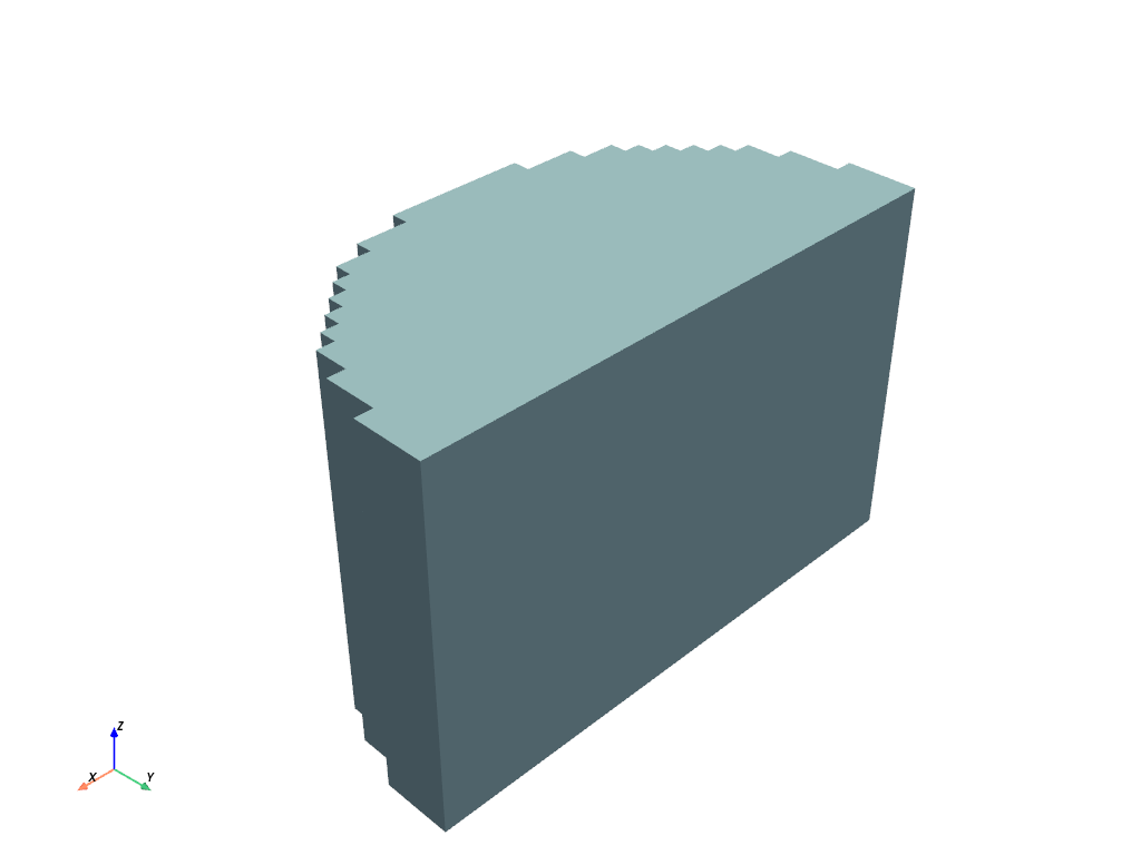
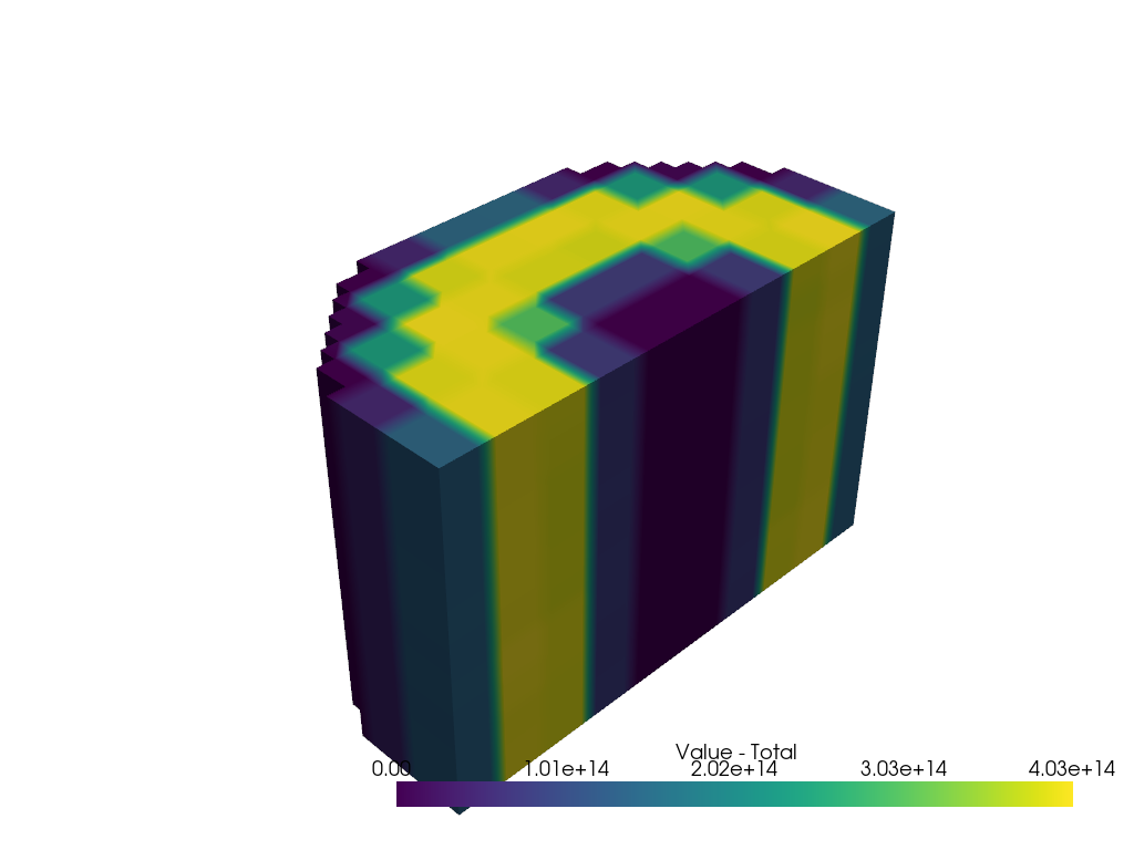
Another handy method from pyvista is the voxelization of stl file and subsequent mapping of pyvista grid onto these voxelized stl
import pyvista as pv
divisions = 50 # increase this will lead to better detail (i.e. smaller size of voxels)
voxelized = stl.voxelize(spacing=stl.length/divisions)

voxelized.clip(normal='y').plot(jupyter_backend='static')
mapped = voxelized.sample(meshtal.mesh[1004].grid)

plotter = pv.Plotter()
plotter.add_mesh(mapped.clip(normal='y'), scalars='Value - Total')
plotter.show(jupyter_backend='static')
Slicing#
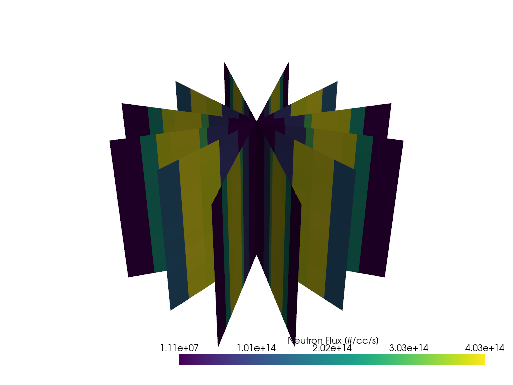
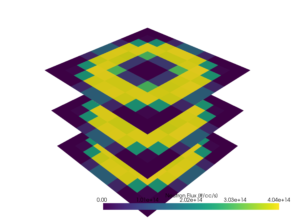
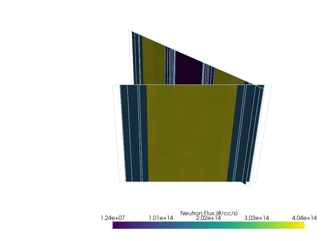
There are different slicing methods that have been defined in F4Enix. All of them produces slices that can be automatically plotted in order to build an atlas.
# Initialize the custom plotter with the mesh and stl
plotter = MeshPlotter(global_mesh, stl=stl)

# There are many default settings that can be modified, e.g.:
# plotter.legend_args['vertical'] = False
# toroidal slicing. It can be done on all the 180 deg or specify the sector
# and origin
toroidal_slices = plotter.slice_toroidal(30)  # 30 deg. increment
# Show the first slice
print(toroidal_slices[0])  # (name of the slice, mesh slice, stl slice)

# Use pyvista native plotter just as an example to show what is the output
pv_plotter = pv.Plotter()
for slices in toroidal_slices:
    mesh_slice = slices[1]
    pv_plotter.add_mesh(mesh_slice)

pv_plotter.show(jupyter_backend='static')
/home/docs/checkouts/readthedocs.org/user_builds/f4enix/envs/developing/lib/python3.10/site-packages/pyvista/core/utilities/helpers.py:394: RuntimeWarning: invalid value encountered in divide
  normal_ = normal_ / np.linalg.norm(normal_)
('theta = 0.0 deg', PolyData (0x778e340f8760)
  N Cells:    100
  N Points:   121
  N Strips:   0
  X Bounds:   0.000e+00, 0.000e+00
  Y Bounds:   -1.300e+03, 1.300e+03
  Z Bounds:   -9.000e+02, 9.000e+02
  N Arrays:   2, PolyData (0x778e340f8820)
  N Cells:    190
  N Points:   138
  N Strips:   0
  X Bounds:   4.000e-01, 4.000e-01
  Y Bounds:   -1.379e+03, 1.379e+03
  Z Bounds:   -9.000e+02, 9.000e+02
  N Arrays:   0)
Normal slicing#
# perform slices normal to the selected axis
horizontal_slices = plotter.slice_on_axis('z', 3)  # 3 slices from max to min
# Show the first slice
print(toroidal_slices[0])  # (name of the slice, mesh slice, stl slice)

# Use pyvista native plotter just as an example to show what is the output
pv_plotter = pv.Plotter()
for slices in horizontal_slices:
    mesh_slice = slices[1]
    pv_plotter.add_mesh(mesh_slice)

pv_plotter.show(jupyter_backend='static')
('theta = 0.0 deg', PolyData (0x778e340f8760)
  N Cells:    100
  N Points:   121
  N Strips:   0
  X Bounds:   0.000e+00, 0.000e+00
  Y Bounds:   -1.300e+03, 1.300e+03
  Z Bounds:   -9.000e+02, 9.000e+02
  N Arrays:   2, PolyData (0x778e340f8820)
  N Cells:    190
  N Points:   138
  N Strips:   0
  X Bounds:   4.000e-01, 4.000e-01
  Y Bounds:   -1.379e+03, 1.379e+03
  Z Bounds:   -9.000e+02, 9.000e+02
  N Arrays:   0)
General slicing#
# General slicing using origin and normals for each slice
# [name, x, y, z, ux, uy, uz]
slices_param = [['slice1', 0, 0, 0, 1, 0, 0],
                ['slice2', 500, 700, 300, 0.5, 0.5, 0]]
general_slices = plotter.slice(slices_param)

# Use pyvista native plotter just as an example to show what is the output
pv_plotter = pv.Plotter()
for slices in general_slices:
    mesh_slice = slices[1]
    stl_slice = slices[2]
    pv_plotter.add_mesh(mesh_slice)
    pv_plotter.add_mesh(stl_slice)

pv_plotter.show(jupyter_backend='static')
Build the Atlas#
pv.global_theme.allow_empty_mesh = True

# Time to plot the slices
meshtal = Meshtal("meshtal")
stl = pv.read("iter1D.stl")

meshtal.readMesh()
mesh = meshtal.mesh[1004].grid

plotter = MeshPlotter(mesh, stl.scale(10))


toroidal_slices = plotter.slice_toroidal(30)  # 30 deg. increment
horizontal_slices = plotter.slice_on_axis("z", 3)  # 3 slices from max to min
global_mesh = plotter.mesh
# Cycle on all the mesh quantities
sections = []
for array_name in global_mesh.array_names:

    # Arbitrary logic can be inserted here
    min_val = 1e6
    max_val = 1e15
    n_colors = 9
    min_max = (min_val, max_val)

    # Plot both the vertical and toroidal slice related to the quantity
    tot_images = []
    for slices in [toroidal_slices, horizontal_slices]:
        # Plot the slices
        images = plotter.plot_slices(
            slices, array_name, n_colors=n_colors, min_max=min_max
        )
        tot_images.extend(images)

    sections.append((array_name, tot_images))

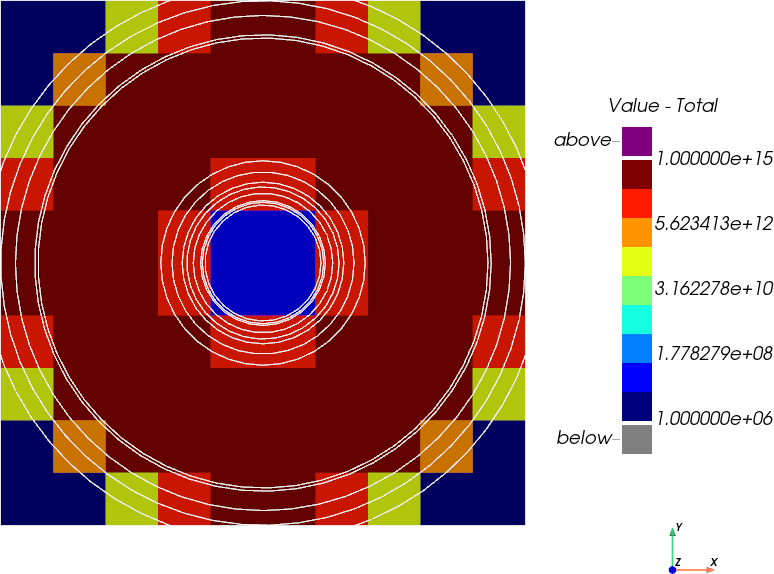
# Show one of the images that will build the atlas
print(sections[0])
print(sections[0][1])
print(sections[0][1][-1])
sections[0][1][-1][1]
('Value - Total', [('theta = 0.0 deg', <PIL.Image.Image image mode=RGB size=816x522 at 0x778E367BA7A0>), ('theta = 30.0 deg', <PIL.Image.Image image mode=RGB size=829x502 at 0x778E340C7CA0>), ('theta = 60.0 deg', <PIL.Image.Image image mode=RGB size=829x502 at 0x778E36A85AE0>), ('theta = 90.0 deg', <PIL.Image.Image image mode=RGB size=220x467 at 0x778E340C7370>), ('theta = 120.0 deg', <PIL.Image.Image image mode=RGB size=829x502 at 0x778E340C52A0>), ('theta = 150.0 deg', <PIL.Image.Image image mode=RGB size=829x502 at 0x778E340C79D0>), ('Pz = -882.0', <PIL.Image.Image image mode=RGB size=774x574 at 0x778E36A87D00>), ('Pz = 0.0', <PIL.Image.Image image mode=RGB size=774x574 at 0x778E3411BF10>), ('Pz = 882.0', <PIL.Image.Image image mode=RGB size=774x574 at 0x778E242B4D00>)])
[('theta = 0.0 deg', <PIL.Image.Image image mode=RGB size=816x522 at 0x778E367BA7A0>), ('theta = 30.0 deg', <PIL.Image.Image image mode=RGB size=829x502 at 0x778E340C7CA0>), ('theta = 60.0 deg', <PIL.Image.Image image mode=RGB size=829x502 at 0x778E36A85AE0>), ('theta = 90.0 deg', <PIL.Image.Image image mode=RGB size=220x467 at 0x778E340C7370>), ('theta = 120.0 deg', <PIL.Image.Image image mode=RGB size=829x502 at 0x778E340C52A0>), ('theta = 150.0 deg', <PIL.Image.Image image mode=RGB size=829x502 at 0x778E340C79D0>), ('Pz = -882.0', <PIL.Image.Image image mode=RGB size=774x574 at 0x778E36A87D00>), ('Pz = 0.0', <PIL.Image.Image image mode=RGB size=774x574 at 0x778E3411BF10>), ('Pz = 882.0', <PIL.Image.Image image mode=RGB size=774x574 at 0x778E242B4D00>)]
('Pz = 882.0', <PIL.Image.Image image mode=RGB size=774x574 at 0x778E242B4D00>)
import tempfile  # To have a scratch directory for the example

# Finally build the atlas. This can be built either from folders containing
# images, where each subfolder is interpreted as a new section, or adding each
# section manually. This second option is recommended since it allows to avoid
# saving the images to disk

# initialize the atlas
atlas = Atlas('Atlas example')

# Decrease the default width of plots (by default they occupy the entire text
# length)
atlas.default_width = atlas.default_width*0.9

# Build one section for each quantity
for arrayname, images in sections:
    atlas.add_section(arrayname, images)

outpath = tempfile.gettempdir()
print(outpath)  # We are saving in the default temporary directory
atlas.save(outpath)
/tmp
Add volume sampling error to CuV Meshtal files#
We are going to calculate the volume with a Monte Carlo integral. A random sample of N points inside a voxel is done, checking for each point if it falls inside the studied cell.
Where \(b_i\) is a random variable that follows a binomial distribution (0 or 1) depending on if the point fell inside the studied cell. \(V_r\) is the partial cell volume over the voxel volume. To know the uncertainty of the estimator V_r we can apply the uncertainty propagation law, as each point is sampled independently.
All \(b_i\) variables follow the same binomial probability distribution, that is, each point has the same chance to fall in the cell. Therefore, \(σ_{(b_i)}^2=σ_b^2\) . Then we can make the sum so:
Where \(σ_b^2\) can be calculated via the variance numeric estimator.
Up to this point, we have seen the same procedure as in many Monte Carlo integrals. For example, that if MCNP as seen in page 2-109 of the MCNP5 Manual I.However, the volume we are calculating is a binomial (0 or 1).
Therefore:
import tempfile  # To have a scratch directory for the example
import os
import pyvista as pv
from f4enix.output.meshtal import Meshtal
from f4enix.output.cuv_sampling_error import add_sampling_error_to_vtk

# Read a meshtal and create a VTK file
meshtal = Meshtal("meshtal_cuv", filetype="CUV")
meshtal.readMesh(norm='ctot')

# write to vtk
tmpdir = tempfile.gettempdir()
outname = 'outfile'
outpath = os.path.join(tmpdir, outname)
meshtal.mesh[44].write(tmpdir, outfile=outname)

# Read the VTK file
grid = pv.read(os.path.join(tmpdir, outname + '.vtr'))

# The amount of sampling points per voxel should be identified from the MCNP input file
# by the user. In this example, it is set to 1000 points per voxel.
grid_with_errors = add_sampling_error_to_vtk(
        grid=grid, cuv_file_path="meshtal_cuv", voxel_sampling_points=1000
    )
grid_with_errors
RectilinearGrid (0x778ddde8bac0)
  N Cells:      16
  N Points:     50
  X Bounds:     -1.000e+01, 1.000e+01
  Y Bounds:     -1.000e+01, 1.000e+01
  Z Bounds:     -5.000e+00, 5.000e+00
  Dimensions:   5, 5, 2
  N Arrays:     3
Apply transformations to FMESH grids#
It is possible to apply transformations to the FMESH tally grids of the meshtal file, given a MCNP TR card. The most standard way is by applying a TR card to a FMESH grid:
from numjuggler import parser
from f4enix.output.meshtal import Meshtal

# Define a -20 degrees rotation around the z axis with MCNP syntax
tr_text = ["*TR1 0 0 0 20.0000 70.0000 90 110.0000 20.0000 90 90 90 0\n"]

## Generate the transformation card
mcnp_transformation = parser.Card(tr_text, 5, 0)
mcnp_transformation.get_values()

# Read the meshtal file
meshtal = Meshtal("meshtal_transform")
meshtal.readMesh()

# Select the mesh to be transformed
mesh_tally_2024 = meshtal.mesh[2024]

# Plot the original mesh
mesh_tally_2024.grid.plot(scalars="Value - Total", show_edges=True, jupyter_backend='static')

# Apply the transformation to the mesh
mesh_tally_2024.apply_transformation(mcnp_transformation)

# Plot the transformed mesh
mesh_tally_2024.grid.plot(scalars="Value - Total", show_edges=True, jupyter_backend='static')
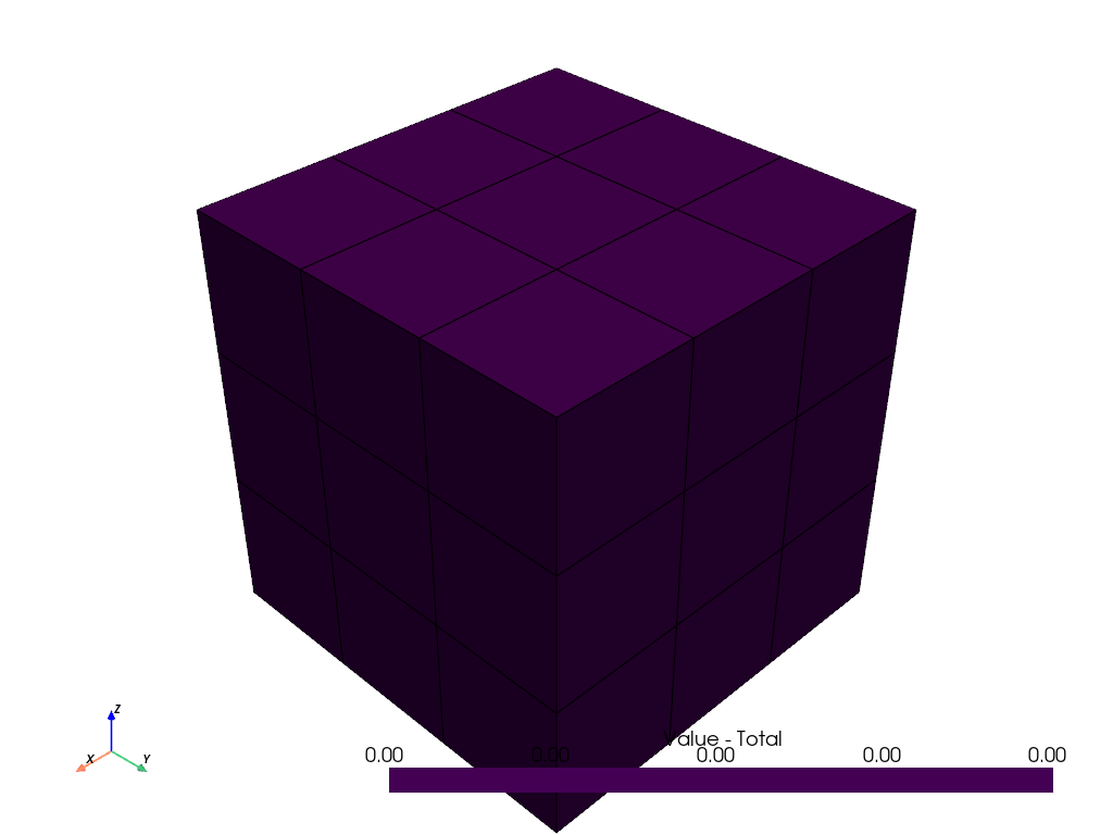
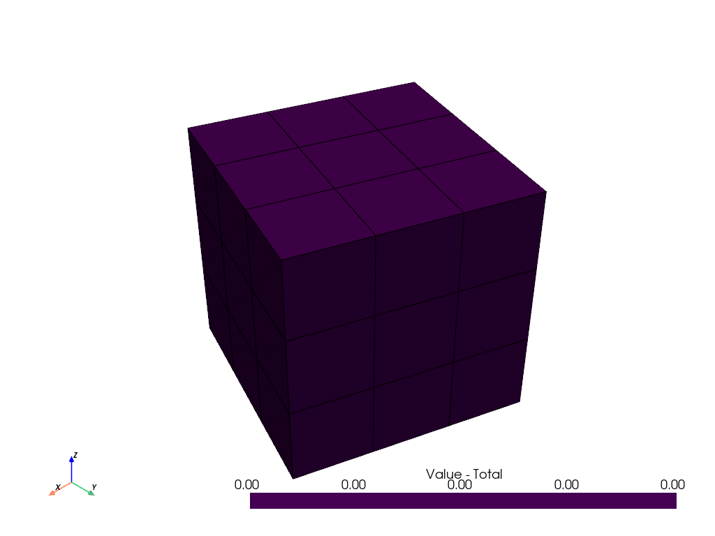
You can also apply multiple transformations to multiple meshes, just by providing a dictionary.
from numjuggler import parser
from f4enix.output.meshtal import Meshtal
# Define a -20 degrees rotation around the z axis with MCNP syntax
tr_rotation_1_text = ["*TR1 0 0 0 20.0000 70.0000 90 110.0000 20.0000 90 90 90 0\n"]
# Define a -45 degrees rotation around the z axis with MCNP syntax, with translation along x
tr_rotation_2_text = ["*TR1 10 0 0 45.0000 45.0000 90 135.0000 45.0000 90 90 90 0\n"]

## Generate the transformation cards
mcnp_transformation_1 = parser.Card(tr_rotation_1_text, 5, 0)
mcnp_transformation_1.get_values()

mcnp_transformation_2 = parser.Card(tr_rotation_2_text, 5, 0)
mcnp_transformation_2.get_values()

# Read the meshtal file
meshtal = Meshtal("meshtal_transform")
meshtal.readMesh()

dict_transformation = {2024: mcnp_transformation_1,
                       2124: mcnp_transformation_2}

meshtal.transform_multiple_fmesh(dict_transformation)

# Select the mesh with the first transformation
mesh_tally_2024 = meshtal.mesh[2024]

# Plot the transformed mesh
mesh_tally_2024.grid.plot(scalars="Value - Total", show_edges=True, jupyter_backend='static')

# Select the mesh with the second transformation
mesh_tally_2124 = meshtal.mesh[2124]

# Plot the transformed mesh
mesh_tally_2124.grid.plot(scalars="Value - Total", show_edges=True, jupyter_backend='static')
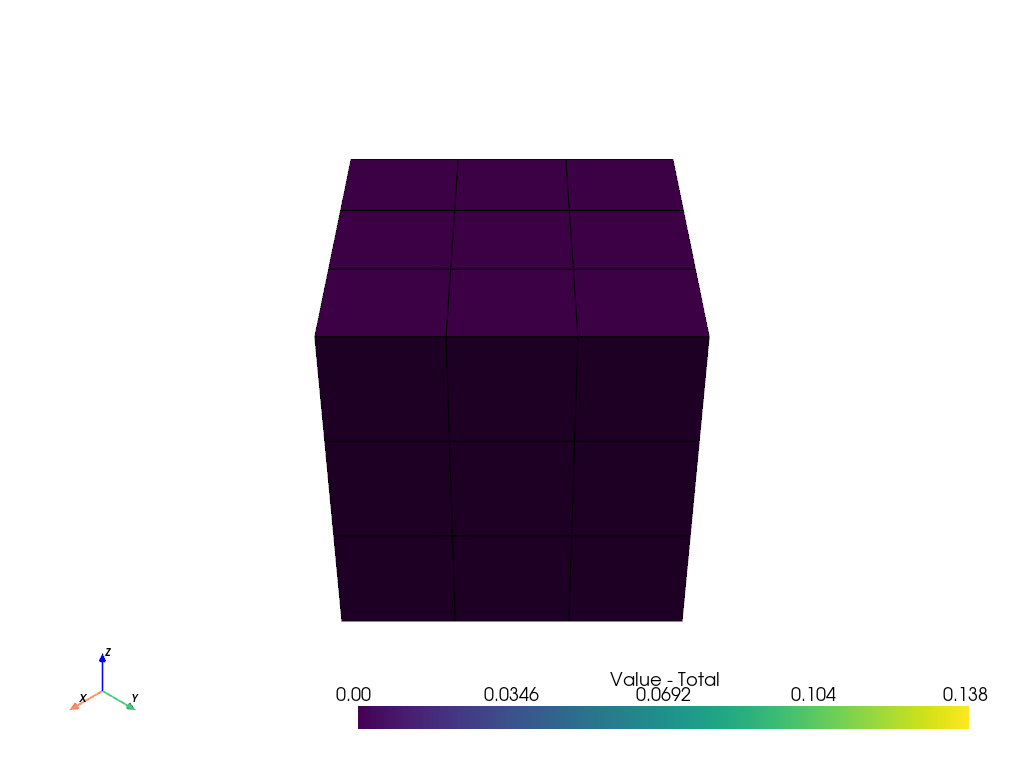
Moreover, you can provide F4Enix with an Input object and let F4Enix transform all FMESH tallies according to the corresponding tr=… labels assigned to each FMESH card in the input
from f4enix.input.MCNPinput import Input
from f4enix.output.meshtal import Meshtal

# Read the meshtal file
meshtal = Meshtal("meshtal_transform")
meshtal.readMesh()

inp = Input.from_input("transforms.i")

meshtal.transform_fmesh(inp)