
Handling irradiation scenarios#
Nuclides and Pulses#
The basic units on which F4Enix relies to operate with irradiation scenarios are the Nuclide and Pulse classes. A Nuclide only mandatory attribute is the zaid but it can support much more information.
from f4enix.core.irradiation import Nuclide

nuclide1 = Nuclide(zaid=1001)
nuclide2 = Nuclide(element='Fe', isotope=56)
for n in [nuclide1, nuclide2]:
    print(n.write_to_formula())
    print(n.write_to_int_string())
/home/docs/checkouts/readthedocs.org/user_builds/f4enix/envs/stable/lib/python3.10/site-packages/tqdm/auto.py:21: TqdmWarning: IProgress not found. Please update jupyter and ipywidgets. See https://ipywidgets.readthedocs.io/en/stable/user_install.html
  from .autonotebook import tqdm as notebook_tqdm
H1
1001
Fe56
26056
Additional data includes library (for parent isotopes of d1suned), metastable flags and IRS flags. Special flags conventions:
Flag |
Formula tag |
Int tag |
|---|---|---|
IRS |
|
|
metastable |
|
|
nuclide = Nuclide(1001, lib="91c", metastable=True, IRS_active=True)
print(nuclide.write_to_formula())
print(nuclide.write_to_int_string())
irsH1m.91c
9991001900.91c
A Nuclide can also be read from the same strings that can produce
print(Nuclide.from_formula("Mo99m.80c"))
print(Nuclide.from_int_string("1001.91c"))
Mo99m.80c
H1.91c
A Pulse instead represents a basic pulse in an irradiation scenario. It is defined by
an intensity and a time interval that can be expressed in different units.
from f4enix.core.irradiation import Pulse
from f4enix.core.constants import TIME_UNITS

pulse = Pulse(2, 2.5e10, TIME_UNITS.MONTH)
print(pulse)
print(f'seconds: {pulse.time}') # internally the time is always stored in seconds
Pulse(time=2.0 TIME_UNITS.MONTH, intensity=25000000000.0)
seconds: 5259666.666666667
Irradiation Scenario#
Starting from a collection of pulses, an irradiation scenario can be built.
from f4enix.core.irradiation import IrradiationScenario

pulses = (
    [Pulse(1, 1e10, TIME_UNITS.DAY), Pulse(2, 0, TIME_UNITS.DAY)]*4 +
    [Pulse(1, 1e11, TIME_UNITS.HOUR)] +
    [Pulse(2, 5e10, TIME_UNITS.HOUR)]*3
)

irr_scenario = IrradiationScenario(pulses)
irr_scenario.pulses
[Pulse(time=1.0 TIME_UNITS.DAY, intensity=10000000000.0),
 Pulse(time=2.0 TIME_UNITS.DAY, intensity=0),
 Pulse(time=1.0 TIME_UNITS.DAY, intensity=10000000000.0),
 Pulse(time=2.0 TIME_UNITS.DAY, intensity=0),
 Pulse(time=1.0 TIME_UNITS.DAY, intensity=10000000000.0),
 Pulse(time=2.0 TIME_UNITS.DAY, intensity=0),
 Pulse(time=1.0 TIME_UNITS.DAY, intensity=10000000000.0),
 Pulse(time=2.0 TIME_UNITS.DAY, intensity=0),
 Pulse(time=1.0 TIME_UNITS.HOUR, intensity=100000000000.0),
 Pulse(time=2.0 TIME_UNITS.HOUR, intensity=50000000000.0),
 Pulse(time=2.0 TIME_UNITS.HOUR, intensity=50000000000.0),
 Pulse(time=2.0 TIME_UNITS.HOUR, intensity=50000000000.0)]
Additionally, the IrradiationScenario class can also be initialized from an existing
FISPACT-II input or legacy d1stime script input with the methods:
IrradiationScenario.from_legacy_d1stime('path_to_file')
and
IrradiationScenario.from_fispact('path_to_file')
By default, a unique cooling time at 0s is added to the irradiation scenario.
This can be changed using the set_cooling_times() method that allows to define times relative
to each other or absolute.
# times relative to each other
irr_scenario.set_cooling_times([(1, TIME_UNITS.SECOND), (3, TIME_UNITS.SECOND)], absolute=False)
print('Relative times:')
print(irr_scenario.cooling_times)
print(irr_scenario.cooling_labels) # always expressed as absolute times

irr_scenario.set_cooling_times([(1, TIME_UNITS.SECOND), (3, TIME_UNITS.SECOND)])

print('\nAbsolute times:')
print(irr_scenario.cooling_times)
print(irr_scenario.cooling_labels) # always expressed as absolute times
Relative times:
[Pulse(time=1.0 TIME_UNITS.SECOND, intensity=0.0), Pulse(time=3.0 TIME_UNITS.SECOND, intensity=0.0)]
['1.0s', '4.0s']

Absolute times:
[Pulse(time=1.0 TIME_UNITS.SECOND, intensity=0.0), Pulse(time=2.0 TIME_UNITS.SECOND, intensity=0.0)]
['1s', '3s']
Also, independently on how the scenario was generated, it is possible to retrieve the irradiation scenario in a “collapsed” format where the repetition of pulse sequences are automatically recognized
irr_scenario.get_collapsed_table()
| Intensity | ||
|---|---|---|
| Repetition | Time | |
| 4 | 1.0 d | 1.000000e+10 |
| 2.0 d | 0.000000e+00 | |
| 1 | 1.0 h | 1.000000e+11 |
| 3 | 2.0 h | 5.000000e+10 |
Time correction factors calculation#
When using a Direct 1 Step (D1S) approach for the calculation of shut down dose rates, time correction factors are required. These factors are computed recursively at each irradiation pulse and for each Nuclide as:
where:
\(\lambda\) is the decay constant of the radioactive nuclide
\(\Delta t_i\) is the duration of the \(i\)-th pulse
\(I\) is the intensity of the neutron source at the \(i\)-th pulse
\(\mathrm{norm}\) is an arbitrary normalization factor
F4Enix allows to compute these factors with the TCF_Computer class. Decay constants are computed with data taken from decay2020 decay library downloadable from the FISPACT website. These values can be recalled with ad hoc get methods:
from f4enix.core.irradiation import TCF_Computer

tcf_computer = TCF_Computer()  # mainly loads the decay data

# Get a lambda or half life value for a single nuclide
nuclide = Nuclide.from_formula("Co60")
lambda_val = tcf_computer.get_lambda(nuclide)
half_life_val = tcf_computer.get_half_life(nuclide)

print(f'Lambda for Co-60: {lambda_val} 1/s')
print(f'Half-life for Co-60: {half_life_val} s')
Lambda for Co-60: 4.167050502344595e-09 1/s
Half-life for Co-60: 166340000.0 s
While the time correction factors can be computed for different isotopes at the same time. Factors will be computed at each cooling time specified in the irradiation scenario.
nuclides = [Nuclide.from_formula("Co60"), Nuclide.from_formula("Co60m")]

tcf_results = tcf_computer.compute_correction_factors(irr_scenario, nuclides, norm=1e10)
tcf_results
array([[2.03637835e-03, 4.99448453e+00],
       [2.03637834e-03, 4.98347184e+00]])
# if needed, it can be organized as a DataFrame
import pandas as pd
df = pd.DataFrame(tcf_results)
df.columns = [nuclide.write_to_formula() for nuclide in nuclides]
df.index = irr_scenario.cooling_labels
df
| Co60 | Co60m | |
|---|---|---|
| 1s | 0.002036 | 4.994485 |
| 3s | 0.002036 | 4.983472 |
Spectra#
F4Enix also offers a Spectra class that allows to interface with FISPACT and other formats. Additionally, it provides handy plotting methods for quick analyses.
Generating spectra#
Spectra can be initialized either directly providing the values or for instance reading a FISPACT FLUXES file.
import numpy as np
from f4enix.core.spectra import Spectra
from f4enix.core.egroups import GROUP_STRUCTURES

# get energy bins from the F4Enix library
g709 = GROUP_STRUCTURES['CCFE-709']
vitamin_j_175 = GROUP_STRUCTURES['VITAMIN-J-175']

# create a spectra with random values (it will be automatically normalized)
spectra1 = Spectra(
    ebins=vitamin_j_175,
    spectra_values=np.random.rand(len(vitamin_j_175) - 1) * 100,
    name="random_spectra",
)

# parse from FLUXES file, energy bins are not given in the fluxes file
spectra2 = Spectra.from_fispact(g709, 'FLUXESS')

# quick plotting of one or more spectra, optional plot by unit lethargy
spectra1.plot(add_spectra=[spectra2], lethargy=True)
WARNING:root:Spectra values must be normalized to 1. Current sum: 8262.35925493946 Normalizing automatically.
(<Figure size 640x480 with 1 Axes>,
 <Axes: title={'center': 'Spectra comparison'}, xlabel='Energy (MeV)', ylabel='Spectra by unit lethargy'>)
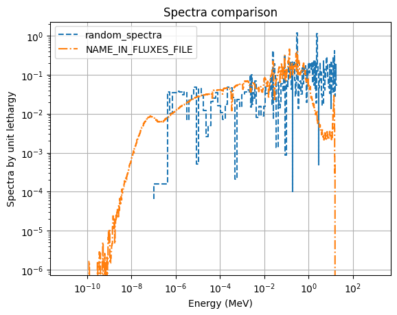
spectra can later be exported to different formats.
from tempfile import TemporaryDirectory
import os

with TemporaryDirectory() as temp_dir:
    # print to "arb_flux" FISPACT format
    spectra1.to_arb_flux_file(temp_dir)
    # print to "FLUXESS" FISPACT format, wall load set to 1
    spectra1.to_fispact_fluxes(temp_dir)
    # print a FISPACT input ready for running the 'condense' utility
    spectra1.print_condensed_inp(temp_dir)
    # print a FISPACT input ready for running the 'collapse' utility
    spectra1.print_collapse_inp(temp_dir)

    for file in os.listdir(temp_dir):
        print(file)
random_spectra
condense.i
collapse.i
arb_flux_random_spectra.txt