
CDGS production#
These examples are related to the production of a Common Decay Gamma Source (CDGS) file starting from a cloud point (often coming from a flunet calculation)
The interpolation#
The starting point to create CDGS is often a cloud point (representing the centroids of a mesh) that have information on the specific atomic density of each radio-isotope of interest and volume in each cell. This information needs to be translated into a structured mesh.
To do so, there are two main thing to decide:
the bin sizes
how to interpolate the cloud point on the new mesh
These two main points are controlled respectively by the
InterpolationKernel and MeshDefinition object families
MeshDefinition#
There are three concrete MeshDefinition children, each controlling how the structured grid is built from the cloud point:
Class |
What you provide |
How the voxel size is determined |
|---|---|---|
|
|
Average nearest-neighbour distance × factor |
|
|
Fixed bin size you specify directly |
|
|
bbox extent / n_voxels per axis |
All three accept an optional bbox dict (x_min, x_max, y_min, y_max, z_min, z_max) to override the automatic bounding box.
The following shows an example of these definition can change significantly the mesh that will be produced
inside the CDGS object
import pandas as pd
import pyvista as pv
from f4enix.output.cdgs import MeshByAverageDistance, MeshByBinSize, MeshByNumberOfVoxels

# Read the same cloud point used in the rest of the notebook
source_activity = pd.read_csv('activity_example1.csv')
source_activity.columns = source_activity.columns.str.strip()
coords = source_activity[['x', 'y', 'z']].values

bbox = {
    "x_min": coords[:, 0].min(),
    "x_max": coords[:, 0].max(),
    "y_min": coords[:, 1].min(),
    "y_max": coords[:, 1].max(),
    "z_min": coords[:, 2].min(),
    "z_max": coords[:, 2].max(),
}

definitions = {
    "MeshByAverageDistance(factor=10)": (MeshByAverageDistance(factor=10)),
    "MeshByBinSize(bin_size=(50, 60, 50))": (MeshByBinSize(bin_size=(50, 60, 50))),
    "MeshByNumberOfVoxels(n_voxels=(10,5,10))": (MeshByNumberOfVoxels(n_voxels=(10, 5, 10), bbox=bbox)),
}

for mesh_name, mesh_def in definitions.items():
    print(f"\nBuilding mesh: {mesh_name}")
    mesh = mesh_def._build_grid(coords)
    print(mesh)
/home/docs/checkouts/readthedocs.org/user_builds/f4enix/envs/latest/lib/python3.10/site-packages/tqdm/auto.py:21: TqdmWarning: IProgress not found. Please update jupyter and ipywidgets. See https://ipywidgets.readthedocs.io/en/stable/user_install.html
  from .autonotebook import tqdm as notebook_tqdm
Building mesh: MeshByAverageDistance(factor=10)
StructuredGrid (0x7cbbaf17d4e0)
  N Cells:      968
  N Points:     1587
  X Bounds:     -7.447e-02, 7.447e-02
  Y Bounds:     -2.626e-01, -2.508e-01
  Z Bounds:     7.896e-01, 9.384e-01
  Dimensions:   23, 3, 23
  N Arrays:     0

Building mesh: MeshByBinSize(bin_size=(50, 60, 50))
StructuredGrid (0x7cbbaf17c880)
  N Cells:      1
  N Points:     8
  X Bounds:     -2.507e+01, 2.507e+01
  Y Bounds:     -3.026e+01, 2.975e+01
  Z Bounds:     -2.421e+01, 2.594e+01
  Dimensions:   2, 2, 2
  N Arrays:     0

Building mesh: MeshByNumberOfVoxels(n_voxels=(10,5,10))
StructuredGrid (0x7cbbaf17cdc0)
  N Cells:      500
  N Points:     726
  X Bounds:     -7.111e-02, 7.111e-02
  Y Bounds:     -2.592e-01, -2.541e-01
  Z Bounds:     7.930e-01, 9.350e-01
  Dimensions:   11, 6, 11
  N Arrays:     0
InterpolationKernel#
There are two concrete InterpolationKernel children. Both share the same neighbour search strategy (a sphere around each source point) but differ in how activity is distributed to the neighbours:
Class |
Key parameter(s) |
Neighbour search |
Activity distribution |
|---|---|---|---|
|
|
sphere of fixed |
uniform — each neighbour receives an equal share |
|
|
same as |
inverse-distance weighted — closer neighbours receive proportionally more |
It is important to notice that both these methods will always conserve locally (how local depends on the interpolation sphere dimension) and globally the total activity.
n_voxels is the more practical option: the search radius is set automatically as a multiple of the mesh voxel size, so it adapts when you change the MeshDefinition.
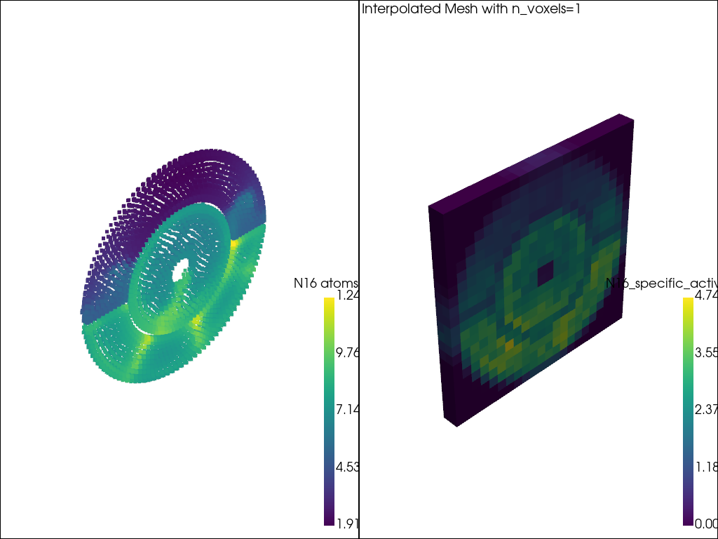
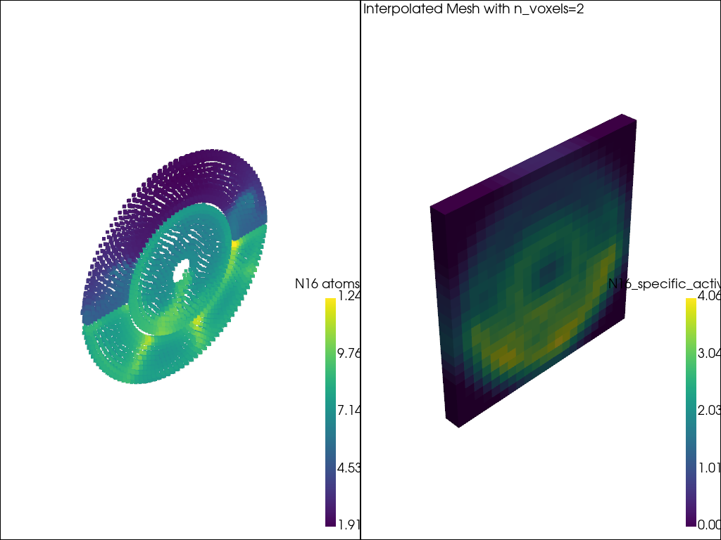
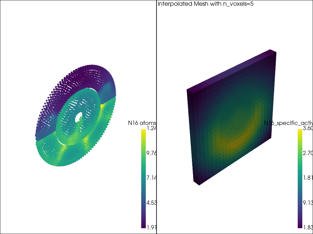
The following example show the effect of using different radius searches on the final interpolated results.
import pandas as pd
from f4enix.output.cdgs import CDGS, SphereKernel, MeshByAverageDistance
from f4enix.output.cdgs.cdgs import ACTIVITY_TAG

source_activity = pd.read_csv('activity_example1.csv')
source_activity.columns = source_activity.columns.str.strip()  # Strip whitespace from column names
cloudpoint = pv.PolyData(source_activity[['x', 'y', 'z']].values)
cloudpoint['N16 atoms/m3'] = source_activity['n16'].values

for n_voxel in [1, 2, 5]:
    cdgs = CDGS.from_cloud_point(
        'activity_example1.csv',
        {"N16": "n16"},
        interpolation_kernel=SphereKernel(n_voxels=n_voxel),
        mesh_definition=MeshByAverageDistance(factor=10),
        col_names={"x": "x", "y": "y", "z": "z", "vol": "cell-volume"}
        )

    interpolated_mesh = cdgs.mesh

    # plotting
    plotter = pv.Plotter(shape=(1, 2))

    plotter.subplot(0, 0)
    plotter.add_mesh(
        cloudpoint,
        scalars='N16 atoms/m3',
        scalar_bar_args={"vertical": True},
    )


    plotter.subplot(0, 1)
    plotter.add_mesh(
        cdgs.mesh,
        scalars=f'N16{ACTIVITY_TAG}',
        scalar_bar_args={"vertical": True},
    )
    plotter.add_text(f"Interpolated Mesh with n_voxels={n_voxel}", font_size=12)

    plotter.show(jupyter_backend="static")
2026-07-21 09:15:36.221 ( 2.758s) [ 7CBC10BDAB80]vtkXOpenGLRenderWindow.:1460 WARN| bad X server connection. DISPLAY=
The CDGS object#
As seen above, the creation of a regular mesh and interpolation happens directly inside the
CDGS object. The data is stored in a pyvista grid and can be further manipulated if needed. In addition to the interpolated atomic density, also the activity is computed and stored in the mesh.
# Create a CDGS object from the cloud point data
cdgs = CDGS.from_cloud_point(
    'activity_example1.csv',
    {"N16": "n16", "O19": "o19"},
    interpolation_kernel=SphereKernel(n_voxels=1),
    mesh_definition=MeshByAverageDistance(factor=10),
    col_names={"x": "x", "y": "y", "z": "z", "vol": "cell-volume"},
    e_bins=None, # If energy bins are not set, emission lines will be used
    particle="gamma" # either gamma or neutron
)
cdgs
CDGS(mesh=StructuredGrid (0x7cbbaedc07c0)
  N Cells:      968
  N Points:     1587
  X Bounds:     -7.447e-02, 7.447e-02
  Y Bounds:     -2.626e-01, -2.508e-01
  Z Bounds:     7.896e-01, 9.384e-01
  Dimensions:   23, 3, 23
  N Arrays:     6, energy_type=CDGS_ENERGY_TYPE.LINE, isotopes=['N16', 'O19'], particle=gamma, cooling_time=0.0)
# Info is stored in a pyvista object
print(cdgs.mesh.array_names)
cdgs.mesh
['N16_specific_activity [Bq/m3]', 'N16_specific_atom_density [atom/m3]', 'O19_specific_activity [Bq/m3]', 'O19_specific_atom_density [atom/m3]', 'N16_intensity [ph/s]', 'O19_intensity [ph/s]']
StructuredGrid (0x7cbbaedc07c0)
  N Cells:      968
  N Points:     1587
  X Bounds:     -7.447e-02, 7.447e-02
  Y Bounds:     -2.626e-01, -2.508e-01
  Z Bounds:     7.896e-01, 9.384e-01
  Dimensions:   23, 3, 23
  N Arrays:     6
# Emission lines are availables also for the combination of radioisotopes
cdgs.all_df
| lines | intensities | isotope | |
|---|---|---|---|
| 10 | 109900.0 | 0.030000 | O19 |
| 11 | 197200.0 | 0.958000 | O19 |
| 0 | 986500.0 | 0.000035 | N16 |
| 12 | 1357000.0 | 0.541000 | O19 |
| 13 | 1444000.0 | 0.030000 | O19 |
| 14 | 1554000.0 | 0.014000 | O19 |
| 15 | 1597000.0 | 0.000300 | O19 |
| 1 | 1755000.0 | 0.001400 | N16 |
| 2 | 1954800.0 | 0.000400 | N16 |
| 16 | 2582000.0 | 0.000300 | O19 |
| 3 | 2741500.0 | 0.008400 | N16 |
| 4 | 2822500.0 | 0.000013 | N16 |
| 17 | 4179000.0 | 0.001300 | O19 |
| 5 | 6048200.0 | 0.000130 | N16 |
| 6 | 6129170.0 | 0.688000 | N16 |
| 7 | 6915500.0 | 0.000400 | N16 |
| 8 | 7115150.0 | 0.050000 | N16 |
| 9 | 8869200.0 | 0.000800 | N16 |
# Or singularly for each isotope
for isotope, values in cdgs.isotopes.items():
    print(f"\nIsotope: {isotope}")
    print(values)
Isotope: N16
{'lines': array([ 986500., 1755000., 1954800., 2741500., 2822500., 6048200.,
       6129170., 6915500., 7115150., 8869200.]), 'intensities': array([3.50000048e-05, 1.39999744e-03, 3.99999760e-04, 8.39999840e-03,
       1.29999664e-05, 1.29999664e-04, 6.88000000e-01, 3.99999760e-04,
       4.99999872e-02, 7.99999520e-04])}

Isotope: O19
{'lines': array([ 109900.,  197200., 1357000., 1444000., 1554000., 1597000.,
       2582000., 4179000.]), 'intensities': array([2.99999616e-02, 9.58000000e-01, 5.40999844e-01, 2.99999616e-02,
       1.40000204e-02, 2.99999616e-04, 2.99999616e-04, 1.29999642e-03])}
Cooling time can be set by the user and will update the values in the CDGS. If a new cooling time is set, the decay of radioisotopes is always computed starting from shutdown activity
print('Cooling time set to 0 seconds by default:')
print(f'{cdgs.get_total_intensity("all"):.2e} photons/s')

cdgs.cooling_time = 100  # Set cooling time to 100 seconds

print('Cooling time set to 100 seconds:')
print(f'{cdgs.get_total_intensity("all"):.2e} photons/s')
Cooling time set to 0 seconds by default:
4.09e+06 photons/s
Cooling time set to 100 seconds:
4.42e+04 photons/s
Helper methods are provided to dump the data either in .vtk or .cdgs (ASCII) format.
import tempfile
tmp_dir = tempfile.gettempdir()

cdgs.to_vtk(tmp_dir + "/cdgs_export.vtk")
cdgs.to_cdgs(tmp_dir + "/cdgs_export.cdgs", 'N16')
# Export a source that combines all isotopes in the CDGS object
cdgs.to_cdgs(tmp_dir + "/cdgs_export_all.cdgs", 'all')